Who would you rather date, Bayes Factor or p-value?
An overview of the differences between Frequentist and Bayesian approaches for the hypothesis testing
Table of contents
Introduction
Frequentist vs Bayesian battle is one of the “hot” topics in the statistics world. On the one hand, Bayesians say that the p-value can be uninformative and Frequentists can find statistically significant differences when in fact there are none. On the other hand, Frequentists are confused with the Bayesians’ priors and where they are coming from. In this overview, I will show an example of hypothesis testing for a population proportion using both approaches. Important to note that this post should serve as an overview, rather than selection of “the best” approach. Most of the calculations will be done “by hand” along with R implementations.
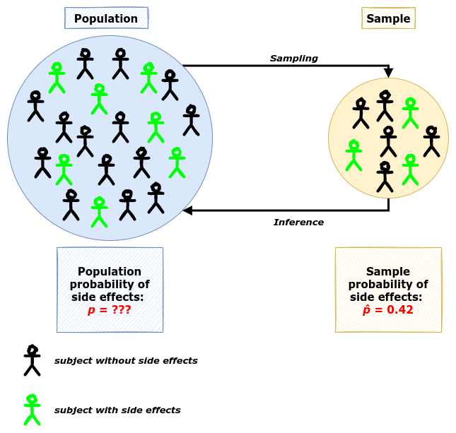
Consider the following example:
Benzodiazepines (also known as tranquilizers) class of drugs are commonly used to treat anxiety. However, such drugs as Xanax can evoke mild side effects like drowsiness or headache pain. Throughout the studies, the side effects were observed at a chance level (around 50% of the time). You believe that the rate of developing side effects is much lower for people under 30 years. You have collected data from 50 young patients with an anxiety disorder who were assigned to Xanax and 21 of them showed the side effects after the drug, \(\hat{p}=0.42\).
Is this result significantly different from a random chance?
Note that numbers are made up.
Frequentist Approach
Null Hypothesis Significance Testing
Let’s start with the Frequentist approach and null hypothesis significance testing (NHST). Under this framework we set the null hypothesis (\(H_0\)) value to some constant, build the desired probability distribution assuming that \(H_0\) is true and then find the probability of observed data in the direction of the alternative hypothesis (\(H_A\)). Direction could be one-sided (less/greater, \(<\) / \(>\), one-tail test) or two-sided (less or greater, \(\neq\), two-tail test). For our example we have:
- \(H_0\): the probability of side effects (SE) after Xanax for young adults is \(50\%\), \(p = 0.5\);
- \(H_A\): the probability of side effects is less than \(50\%\), \(p < 0.5\);
- Significance level \(\alpha=5\%\)
In other words, we build a distribution under the assumption that the probability of side effects is 50% and we want to check if the data we collected (21 out of 50 subjects with side effects) provides enough evidence that it comes from the distribution with another probability (which is less than 50% in our case). The significance level is the threshold value, which is somewhat arbitrary, but conventionally set to 5%. We will reject the null hypothesis if the p-value1 is less than \(\alpha\).
\(\scriptsize n=50\), \(\scriptsize k=21\)
Since our data follows a Binomial distribution we can calculate the probability mass function given the null hypothesis value.
n <- 50
k <- 21
h_0 <- 0.5  # null hypothesis value
x <- 1:n  # sample space
probs <- dbinom(x = x, size = n, p = h_0)  # PMF

light_blue <- "#f5fbfe"
dark_blue <- "#78c2f7"
cols <- ifelse(x <= k, dark_blue, light_blue)

barplot(
  probs, names = x, col = cols,
  main = "PMF Under the Null Hypothesis",
  ylab = "Probability",
  xlab = "Amount of people with side effects (n=50)")
legend(
  "topright", legend = c("p-value"),
  fill = c(dark_blue), bty = "n")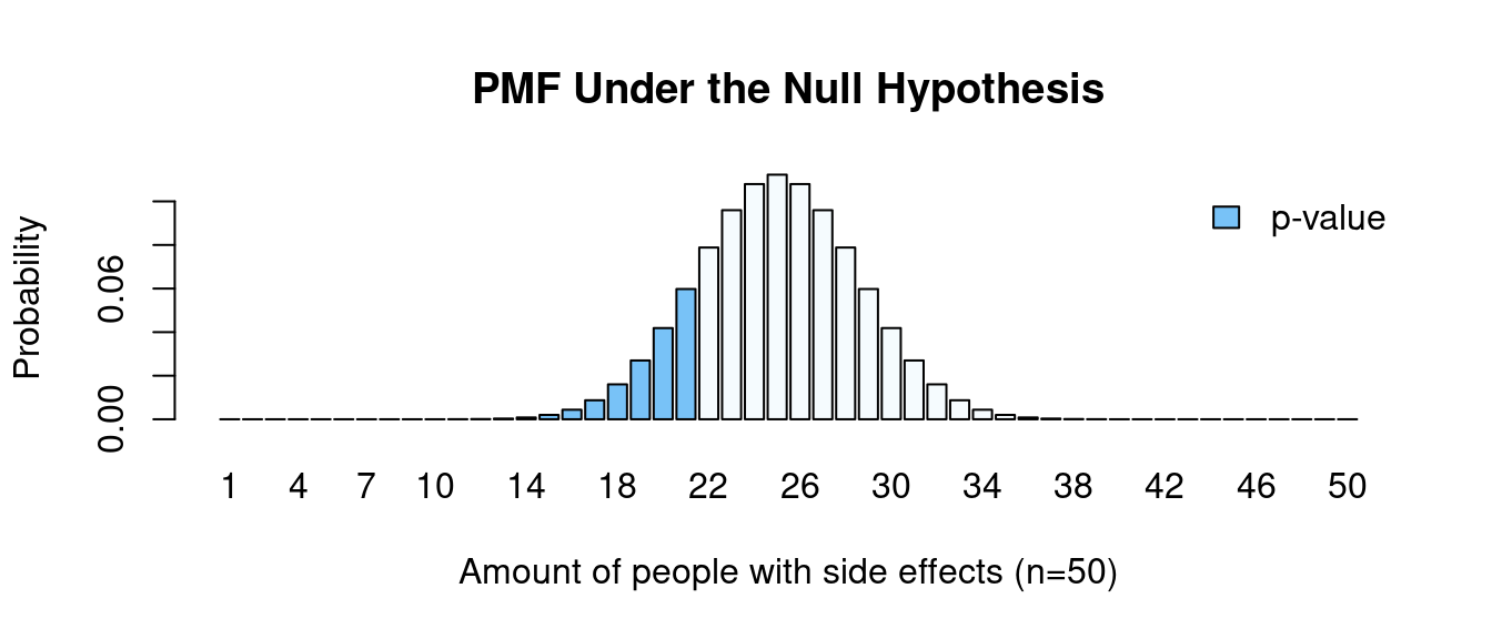
We want to know the probability of obtaining the results as extreme as the results observed. Since we had a one-tail test (\(<\)), the “extreme” results would be obtaining 21 or fewer people with side effects (blue bars).
\[\scriptsize \begin{align*} \text{p-value} &= \sum_{i=0}^k P(X_i) = P(0) + P(1) + ... + P(21) \\ &= \binom{50}{0} \left( \frac{1}{2} \right) ^0 \left( 1 - \frac{1}{2} \right) ^{50-0} + \binom{50}{1}\left( \frac{1}{2} \right) ^1 \left( 1 - \frac{1}{2} \right) ^{50-1} \\ &+ \text{...} + \binom{50}{21} \left( \frac{1}{2} \right) ^{21} \left( 1 - \frac{1}{2} \right) ^{50-21} \\ &\approx 0.161 \end{align*}\]
p_val <- pbinom(q = k, size = n, prob = h_0)
# or
# p_val <- sum(probs[x < k])
cat(p_val)
# 0.161Alternative
binom.test(x = k, n = n, p = h_0, alternative = "less")#
# Exact binomial test
#
# data: k and n
# number of successes = 21, number of trials = 50, p-value = 0.2
# alternative hypothesis: true probability of success is less than 0.5
# 95 percent confidence interval:
# 0.000 0.546
# sample estimates:
# probability of success
# 0.42p-value equals 0.161 so we failed to reject the null hypothesis, meaning that there is not enough evidence to claim that the probability of developing side effects after Xanax for young adults is less than a random chance.
Quiz Question #1. What does p-value tell us?
🅰 Probability that null hypothesis is true, given the data, \(\text{P} (H_0 \text { is true} | \text{Data}) = 16.1\%\)
That is wrong!
🅱 Probability that null hypothesis is false, given the data, \(\text{P} (H_0 \text { is false} | \text{Data}) = 16.1\%\)
That is wrong!
🅲 Probability of observing the data, given that the null hypothesis is true, \(\text{P} (\text{Data} | H_0 \text { is true}) = 16.1\%\)
That is correct!
🅳 Probability of observing the data, given that the null hypothesis is false, \(\text{P} (\text{Data} | H_0 \text { is false}) = 16.1\%\)
That is wrong!
Changing Hypotheses
Here is an interesting phenomenon. We have seen that there is not enough evidence to reject the hypothesis that our data come from a distribution with a probability of success of 0.5. What will happen if we change the hypothesis but keep the idea somewhat similar. Is there enough evidence to claim that the population proportion is greater than 0.4?
- \(H_0\): the probability of side effects (SE) is \(40\%\), \(p= 0.4\);
- \(H_A\): the probability of side effects is greater than \(40\%\), \(p > 0.4\);
- Significance level \(\alpha=5\%\)
h_0 <- 0.4
probs <- dbinom(x = x, size = n, p = h_0)
cols <- ifelse(x >= k, dark_blue, light_blue)

barplot(
  probs, names = x, col = cols,
  main = "PMF Under the Null Hypothesis",
  ylab = "Probability",
  xlab = "Amount of people with side effects (n=50)")
legend(
  "topright", legend = c("p-value"),
  fill = c(dark_blue), bty = "n")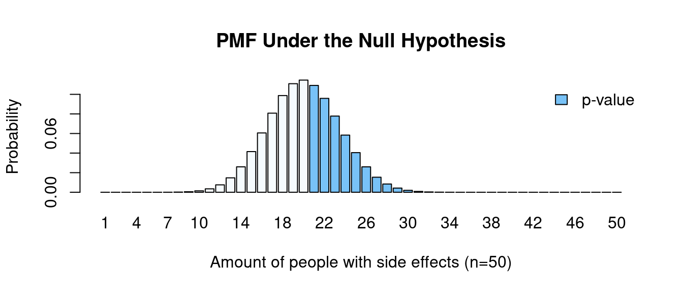
\[\scriptsize \begin{align*} \text{p-value} &= \sum_{i=21}^n P(X_i) = P(21) + P(22) + ... + P(50) \\ &= \binom{50}{21} \left( \frac{4}{10} \right) ^{21} \left( 1 - \frac{4}{10} \right) ^{50-21} + \binom{50}{2} \left( \frac{4}{10} \right) ^{22} \left( 1 - \frac{4}{10} \right) ^{50-22} \\ &+ ... + \binom{50}{50} \left( \frac{4}{10} \right) ^{50} \left( 1 - \frac{4}{10} \right) ^{50-50} \\ &\approx 0.439 \end{align*}\]
p_val <- 1 - pbinom(q = k-1, size = n, prob = h_0)
# or
# p_val <- sum(probs[x >= k])
cat(p_val)
# 0.439Alternative
binom.test(x = k, n = n, p = h_0, alternative = "greater")#
# Exact binomial test
#
# data: k and n
# number of successes = 21, number of trials = 50, p-value = 0.4
# alternative hypothesis: true probability of success is greater than 0.4
# 95 percent confidence interval:
# 0.301 1.000
# sample estimates:
# probability of success
# 0.42Now we calculate the binomial pmf function with the probability of success \(p=0.4\) and the p-value is going to be a sum of probabilities \(\text{P}(x \geq 21)\). We can see that this value is around 44%, which is much higher than our significance level alpha. Again, we failed to reject the null hypothesis, meaning that there is not enough evidence to claim that the probability of developing side effects is higher than 40%.
We were unable to reject the hypothesis that the chances of side effects are 50%, but at the same time, we were unable to reject the hypothesis that the chances are 40%. As we can see, NHST is very sensitive to the null hypothesis you choose. Changing the hypotheses (even if the idea behind them stays quite the same) can lead to contradictory results.
Confidence Intervals
We could also build a Frequentist confidence interval to show our uncertainty about the ratio of side effects. For the large amount of \(n\) in binomial trials, we can say that random variable \(X\) follows a normal distribution with the mean \(\hat{p}\) and standard error \(\sqrt{\frac{\hat{p}(1-\hat{p})}{n}}\).
\[\scriptsize X \sim \mathcal{N} \left( \mu = \hat{p}, SE = \sqrt{\frac{\hat{p}(1-\hat{p})}{n}} \right)\]
Once we have a normal distribution we can easily calculate 95% CI:
\[\scriptsize (1-\alpha) \text{% CI}: \mu \pm Z_{1-\alpha/2} \cdot SE\]
- \(\scriptsize \hat{p} = \frac{k}{n}=0.42\)
- \(\scriptsize Z_{1-0.05/2} = 1.96\)
- \(\scriptsize SE = \sqrt{\frac{0.42(1-0.42)}{50}} \approx 0.07\)
\[\scriptsize 95\text{% CI}: [ 0.283, 0.557 ]\]
p_hat <- k/n
alpha <- 0.05
z_score <- qnorm(p = 1 - alpha/2)
se <- sqrt((k/n * (1-k/n)) / n)
lwr <- p_hat - z_score*se
uppr <- p_hat + z_score*se

cat(
  paste0(
    "95% CI for the proportion: [",
    round(lwr,3), ", ", round(uppr,3), "]"
  )
)
# 95% CI for the proportion: [0.283, 0.557]Quiz Question #2. What can we say according to this CI? Probability that the true value (p) is in the [0.283, 0.557] range is …
🅰 95%, \(\text{P} \left( p \in [0.283, 0.557] \right) = 95\%\)
That is wrong!
🅱 100%, \(\text{P} \left( p \in [0.283, 0.557] \right) = 100\%\)
That is wrong!
🅲 0, \(\text{P} \left( p \in [0.283, 0.557] = 0 \right)\)
That is wrong!
🅳 either 0 or 100%, \(\text{P} \left( p \in [0.283, 0.557] = \{ 0, 100\% \} \right)\)
That is correct!
We are 95% confident that the true probability of side effects lies in the interval \([0.283, 0.557]\). However, we don’t know if our CI has included the true value (it is either has or has not). We can also say, that if we would get more samples of the size 50 and calculated the CI for each of them, 95% of these CIs would hold a true value.
Bayesian Approach
Distinct Hypotheses
Now it is the turn of the Bayesian approach. Under this framework, we can specify two distinct hypotheses and check which one is more likely to be true.
- \(H_1\): the probability of side effects is 50%, \(p=0.5\);
- \(H_2\): the probability of side effects is 40%, \(p=0.4\);
We are going to apply the Bayes rule to calculate the posterior probability after we observed the data.
\[\scriptsize P(\text{Model}|\text{Data}) = \frac{P(\text{Data|Model}) \cdot P(\text{Model})}{P(\text{Data})}\]
- \(P(\text{Data|Model})\) is the likelihood, or probability that the observed data would happen given that model (hypothesis) is true.
- \(P(\text{Model})\) is the prior probability of a model (hypothesis).
- \(P(\text{Data})\) is the probability of a given data. It is also sometimes referred to as normalizing constant to assure that the posterior probability function sums up to one.
- \(P(\text{Model}|\text{Data})\) is the posterior probability of the hypothesis given the observed data.
As we’ve said at the beginning, in previous studies side effects were observed at a chance level, so we may put more “weight” on a prior for the such hypothesis. For example,
Priors:
- \(\scriptsize P(H_1) = 0.75\)
- \(\scriptsize P(H_2) = 0.25\)
Note that the prior probability mass function has to sum up to 1.
Likelihood:
\[\scriptsize \begin{align*} P(k = 21 | H_1 \text{ is true}) &= \binom{n}{k} \cdot P(H_1)^k \cdot (1-P(H_1))^{n-k} \\ &= \binom{50}{21} \cdot 0.5^{21} \cdot (1-0.5)^{50-21} \\ &= 0.0598 \end{align*}\]
\[\scriptsize \begin{align*} P(k = 21 | H_2 \text{ is true}) &= \binom{n}{k} \cdot P(H_2)^k \cdot \left( 1-P(H_2) \right) ^{n-k} \\ &= \binom{50}{21} \cdot 0.4^{21} \cdot (1-0.4)^{50-21} \\ &= 0.109 \end{align*}\]
Posteriors:
\[\scriptsize P(H_1 \text{ is true|}k = 21) = \frac{P(k = 21 | H_1 \text{ is true}) \cdot P(H_1)}{P(\text{k = 21})}\]
\[\scriptsize P(H_2 \text{ is true|}k = 21) = \frac{P(k = 21 | H_2 \text{ is true}) \cdot P(H_2)}{P(\text{k = 21})}\]
\[\scriptsize \begin{align*} P(k=21) &= P(k = 21 | H_1 \text{ is true}) \cdot P(H_1) + P(k = 21 | H_2 \text{ is true}) \cdot P(H_2) \\ &= 0.0598 \cdot 0.75 + 0.109 \cdot 0.25 \\ &= 0.0721 \end{align*}\]
- \(\scriptsize P(H_1 \text{ is true|}k = 21) = 0.622\)
- \(\scriptsize P(H_2 \text{ is true|}k = 21) = 1 - P(H_1 \text{ is true|}k = 21) = 0.378\)
As we can see, the probability of the second hypothesis \(\big( p = 40\% \big)\) equals 37.8%, whereas the probability of the first hypothesis \(\big( p = 50\% \big)\) equals 62.2%.
If we want to check if there is enough evidence against one of the hypotheses, we can also use the Bayes factor2.
\[\scriptsize \begin{align*} \text{BF}(H_2:H_1) &= \frac{\text{Likelihood}_2}{\text{Likelihood}_1} \\ &= \frac{P(k = 21 | H_2 \text{ is true})}{P(k = 21 | H_1 \text{ is true})} \\ &= \frac{\frac{P(H_2 \text{ is true}|k=21) P(k=21)}{P(H_2\text{ is true)}}}{\frac{P(H_1 \text{ is true}|k=21) P(k=21)}{P(H_1\text{ is true)}}} \\ &= \frac{\frac{P(H_2 \text{ is true}|k=21)}{P(H_1\text{ is true}|k=21)}}{\frac{P(H_2)}{P(H_1)}} \\ &= \frac{\text{Posterior Odds}}{\text{Prior Odds}} \end{align*}\]
\[\scriptsize \text{BF}(H_2:H_1)= \frac{\frac{0.646}{0.354}}{\frac{0.5}{0.5}} \approx 1.82\]
To interpret the value we can refer to Harold Jeffreys interpretation table:

Hence we can see there is not enough supporting evidence for \(H_2\) (that the side effects probability is 40%).
priors <- list(h1 = 0.75, h2 = 0.25)
model <- list(h1 = 0.5, h2 = 0.4)
likelihood <- list(
  h1 = dbinom(x = k, size = n, prob = model$h1),
  h2 = dbinom(x = k, size = n, prob = model$h2))
norm_const <- likelihood$h1 * priors$h1 + likelihood$h2 * priors$h2
posterior <- list(
  h1 = likelihood$h1 * priors$h1 / norm_const,
  h2 = likelihood$h2 * priors$h2 / norm_const
)
BF <- likelihood$h2 / likelihood$h1

cat(paste0("Bayes Factor (H2:H1) = ", round(BF,2)))
# Bayes Factor (H2:H1) = 1.82par(mfrow=c(1,3))
barplot(
unlist(priors), col = light_blue,
ylab = "Probability", main = "Priors",
ylim = c(0, 0.8), border = dark_blue)
barplot(
unlist(likelihood), col = light_blue,
main = "Likelihood", border = dark_blue)
barplot(
unlist(posterior), col = light_blue,
main = "Posteriors", ylim = c(0,0.8),
border = dark_blue)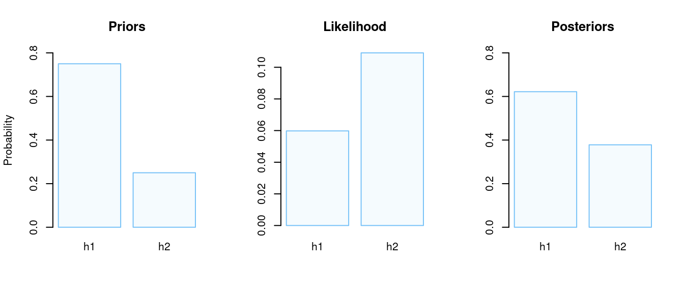
How can we interpret these results? Initially, we believed (based on prior knowledge/intuition/solar calendar/etc.) that the probability of side effects are around the chance level and we applied this by putting more “weight” or prior probability on the first hypothesis. After we have seen the data (21 out of 50 subjects with side effects) we updated our beliefs and got posterior probabilities that were slightly shifted from our initial beliefs. Now the probability that the probability of side effects is around the chance level is around 62% (compared to the initial 75%). But according to the Bayes factor, there is not enough evidence to claim that any of these two hypotheses is more likely to be true.
One might argue that the Bayesian factor is not really part of the Bayesian statistics or it does not represent the whole picture of it. So let us explore what other features of Bayesian statistics exist.
Beta-Binomial Distribution and Credible Intervals
So far we have specified two distinct hypotheses \(H_1\) and \(H_2\). But also we could define the whole prior probability distribution function of an unknown parameter \(p\).
Let’s assume that we have no prior information about the probability of side effects and \(p\) can take any value on the \([0,1]\) range. Or in other words \(p\) follows a uniform distribution \(p \sim \text{Unif}(0,1)\). We are going to replace the Uniform distribution with Beta distribution \(\text{Beta}(\alpha,\beta)\) with parameters \(\alpha=1\), \(\beta=1\), \(p \sim \text{Beta}(1,1)\), which is exactly like the uniform. It just makes calculations (and life) easier since Beta and Binomial distribution3 form a conjugate family4.
Now, in order to find the posterior distribution we can just update the values of the Beta distribution:
- \(\scriptsize \alpha^* = \alpha + k\)
- \(\scriptsize \beta^* = \beta + n - k\)
The expected value of the Beta distribution is:
\[\scriptsize \mathbb{E}(x) = \frac{\alpha}{\alpha+\beta}\]
To summarize:
- Prior: \(\scriptsize p \sim \text{Beta}(\alpha=1,\beta=1)\)
- Likelihood: \(\scriptsize \mathcal{L}( p ) \sim \text{Binom}(n, p)\)
- Posterior: \(\scriptsize p | n,k \sim \text{Beta}(\alpha^*=\alpha + k,\beta^* = \beta + n - k)\)
After we find the posterior distribution we can derive the Bayesian credible interval (CrI) which will tell us the probability of our unknown parameter \(P\). Usually, it is found as the narrowest interval with the desired area (like 0.95).
Code
binom_beta <- function(a, b, n, k){

  x <- seq(from = 0, to = 1, by = 0.005)

  # prior values
  mean_prior <- a/(a+b)
  prior <- dbeta(x = x, shape1 = a, shape2 = b)

  likelihood <- dbinom(x = k, size = n, prob = x)

  # posterior values
  a_new <- a + k
  b_new <- b + n - k
  mean_posterior <- a_new / (a_new+b_new)
  posterior = dbeta(x = x, shape1 = a_new, shape2 = b_new)

  # 94% credible interval
  lwr <- qbeta(p = 0.03, shape1 = a_new, shape2 = b_new)
  uppr <- qbeta(p = 0.97, shape1 = a_new, shape2 = b_new)
  l <- min(which(x >= lwr))
  h <- max(which(x <= uppr))

  par(mfrow=c(1,3))

  plot(
    x, prior, type = "l", lwd = 2, frame.plot=FALSE,
    main = "Prior", ylab = "Density", xlab = "p")
  abline(v = mean_prior, lty = 2, lwd = 1, col = "red")

  plot(
    x, likelihood, type = "l", lwd = 2, frame.plot=FALSE,
    main = "Likelihood", ylab = "", xlab = "p")

  plot(
    x, posterior, type = "l", lwd = 2, frame.plot=FALSE,
    main = "Posterior", ylab = "", xlab = "p|n, k")
  polygon(
    c(x[c(l, l:h, h)]),
    c(0, posterior[l:h], 0),
    col = dark_blue,
    border = 1)
  abline(v = mean_posterior, lty = 2, lwd = 1, col = "red")
  legend(
  "topright", bty = "n",
  legend = c("mean", "94% CrI"),
  col = c("red", NA),
  lty = c(2, NA),
  fill = c("red", dark_blue),
  border = c(NA,dark_blue),
  density = c(0, NA),
  x.intersp=c(1,0.5)
  )

  cat(paste0("n = ", n, "\n"))
  cat(paste0("k = ", k, "\n"))
  cat(paste0("Prior mean: ", round(mean_prior, 3), "\n"))
  cat(paste0("Posterior mean: ", round(mean_posterior, 3), "\n"))
  cat(paste0("94% credible interval: [", round(lwr, 3), ", ", round(uppr, 3), "]", "\n"))
}
binom_beta(a=1, b=1, n=n, k=k) 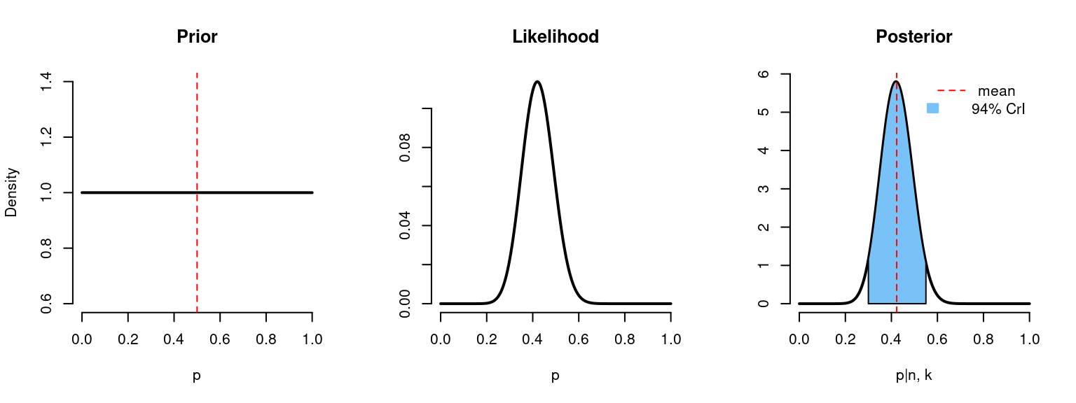
# n = 50
# k = 21
# Prior mean: 0.5
# Posterior mean: 0.423
# 94% credible interval: [0.298, 0.553]
Quiz Question #3. What can we say according to this CrI? Probability that the true value (p) is in the [0.298, 0.553] range is …
🅰 95%, \(\text{P} \left( p \in [0.298, 0.553] = 95\% \right)\)
That is correct!
🅱 100%, \(\text{P} \left( p \in [0.298, 0.553] = 100\%\right)\)
That is wrong!
🅲 0, \(\text{P} \left( p \in [0.298, 0.553] = 0\right)\)
That is wrong!
🅳 either 0 or 100%, \(\text{P} \left( p \in [0.298, 0.553] = \{ 0, 100\% \}\right)\)
That is wrong!
At first, we knew nothing about our parameter \(p\), it could be any value from 0 to 1 with the expected value of 0.5 (prior). After we got 21 out of 50 subjects with side effects we could calculate the probability of obtaining such results under each value of \(p\) in the \([0,1]\) range (likelihood). And finally, we were able to update our probability distribution function to get the posterior probabilities. We see, that given the data, the expected value for the \(p\) is 0.42. The real value of \(p\) is in the range \([0.298, 0.553]\) with the probability of 95% (CrI).
However, flat priors are also called non-informative and they don’t fully match the idea of Bayesian updating. In the example research question, we have said that the probability of side effects is believed to be at a chance level based on the previous data. We can use this information for the prior probability by choosing values \(\alpha = \beta = 10\). In this case, we put more “weight” around the chance level probability.
binom_beta(a=10, b=10, n=n, k=k)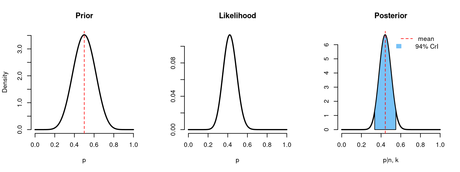
# n = 50
# k = 21
# Prior mean: 0.5
# Posterior mean: 0.443
# 94% credible interval: [0.334, 0.555]
With the relatively large data, posterior distribution relies more on a likelihood, rather than a prior probability distribution. As we can see, posterior distribution has not shifted that much, meaning the priors didn’t have so much weight compared to likelihood.
Now imagine that we have 5 times more observations (with the same ratio 0.42):
binom_beta(a=10, b=10, n=n*5, k=k*5)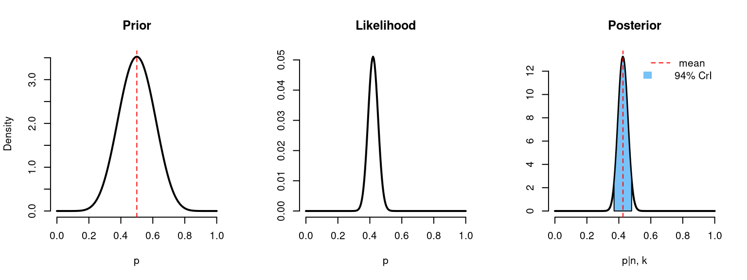
# n = 250
# k = 105
# Prior mean: 0.5
# Posterior mean: 0.426
# 94% credible interval: [0.37, 0.483]
The shape of the posterior distribution looks more like the shape of the likelihood and now the credible interval became narrower, meaning that we have decreased uncertainty about the unknown parameter \(p\).
94% credible intervals may look like a weird choice. But it does not really matter what interval we are choosing (e.g. 95%, 94%, 89%), since it doesn’t have any special meaning (like Frequentists’ CI has). It is just used as an overview of the distribution, but still, to get the full sense of results, Bayesian would use the whole distribution and not just estimates such as mean, quantiles, etc.
Summary
As has been told at the beginning, the purpose of this overview was not to distinguish “the best” approach, but rather to look at their differences. Important to know that both approaches cannot fix the bad experimental design. The key points of each approach can be summarized like this:
| Frequentist Approach | Bayesian Approach |
|---|---|
| Establishes the probability of the data given the model | Establishes the probability of the model given the data |
| Does not rely on prior information about the unknown | Relies on prior information about the unknown (but prior beliefs become less significant as the sample size increases) |
| Sensitive to the null hypothesis | Is not sensitive to hypotheses |
| Estimates the degree of uncertainty using confidence intervals | Estimates the degree of uncertainty using credible intervals |
| Cannot distinguish the probability of a true value in a CI (it is either 0 or 1) | Can distinguish the probability of a true value in a CrI |
Additional Resources
If you would like to learn more about Frequentist and Bayesian approaches, here are some more resources:
- An Introduction to Bayesian Thinking. A Companion to the Statistics with R Course, Merlise Clyde, Mine Cetinkaya-Rundel, Colin Rundel, David Banks, Christine Chai, Lizzy Huang, 2020: Online book
- An Introduction to Bayesian Data Analysis for Cognitive Science, Bruno Nicenboim, Daniel Schad, and Shravan Vasishth, 2020: Online book
- Statistics with R Specialization by Duke University: Coursera specialization
- Bayesian Statistics: From Concept to Data Analysis by University of California, Santa Cruz: Coursera course
- Bayesian statistics: a comprehensive course: YouTube videos
- Keysers, C., Gazzola, V. & Wagenmakers, EJ. Using Bayes factor hypothesis testing in neuroscience to establish evidence of absence. Nat Neurosci 23, 788–799 (2020). https://doi.org/10.1038/s41593-020-0660-4