How do CART models work
Example for the Binary Classification Problem
Cover image credit: Elliott Engelmann
Table of contents
- What is CART?
- Information Gain and Entropy
- Growing a Tree
- Let Computer Do the Math
- Numerical Explanatory Variables
- Other Splitting Metrics
- Summary
- References
# r import
library(tidyverse)
library(knitr)
library(kableExtra)
library(Rgraphviz)
library(rpart)
library(rattle)
library(reticulate)
# python import
import pandas as pd
from sklearn import tree
import matplotlib.pyplot as pltWhat is CART?
Classification and Regression Trees (or CART for short) is a type of supervised machine learning algorithm [1] that is mostly used in classification problems [2], but can be applied for regression problems [3] as well. It can handle both categorical and numerical input variables.
In this tutorial, we are going to go step-by-step and build a tree for the classification problem. A way to solve the regression problem will be discussed at the end.
Imagine that we have medical data about patients and we have two drugs (Drug A and Drug B) that work differently for each patient based on their health metrics. We have such data for 15 patients. Now, the 16th patient comes in and we want to assign a drug to him based on this information. You can load the sample data set here.
patients_df <- read_csv("DecisionTree_SampleData.csv")
kable(patients_df, format = "markdown", caption = "<b>Patients Data</b>")| Patient ID | Gender | BMI | BP | Drug |
|---|---|---|---|---|
| p01 | M | not normal | not normal | Drug A |
| p02 | M | not normal | normal | Drug B |
| p03 | M | not normal | not normal | Drug A |
| p04 | M | normal | not normal | Drug A |
| p05 | M | not normal | not normal | Drug A |
| p06 | F | not normal | normal | Drug B |
| p07 | F | normal | not normal | Drug A |
| p08 | F | not normal | normal | Drug B |
| p09 | M | not normal | not normal | Drug A |
| p10 | M | normal | not normal | Drug A |
| p11 | F | not normal | not normal | Drug B |
| p12 | F | normal | normal | Drug B |
| p13 | F | normal | normal | Drug B |
| p14 | M | normal | not normal | Drug B |
| p15 | F | not normal | normal | Drug B |
| p16 | M | not normal | not normal | ??? |
Our decision tree is going to look something like this:
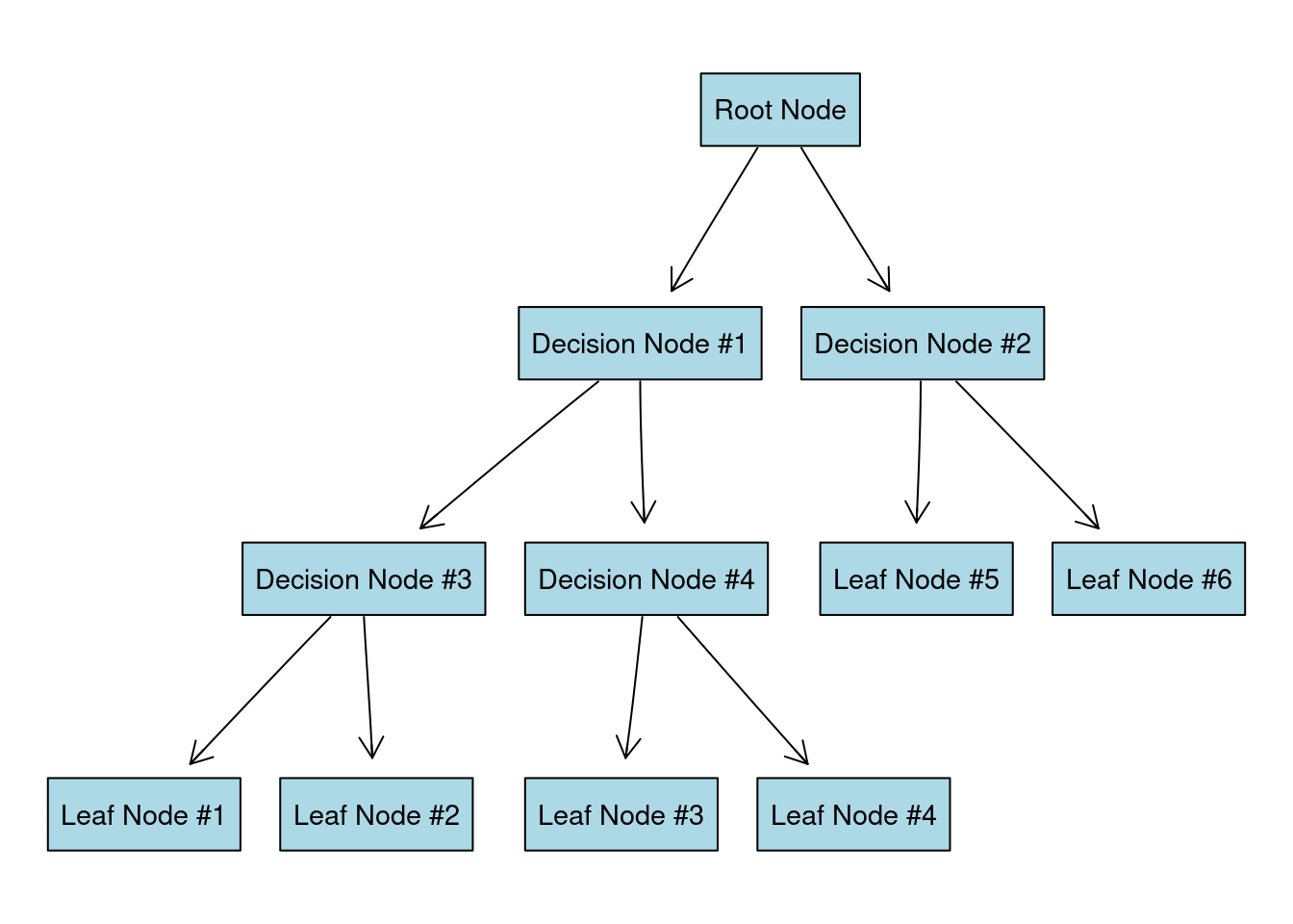
In case you are wondering why is it called “a tree”, you have to look at it upside down:
Imagine that all our data is located at the root node of the tree. We want to split the data by most significant features (that will create new decision nodes) until we reach the leaf nodes with the most homogeneous target possible (ideally just one class is present in each leaf node).
The question is how do we split the data at each node?
Information Gain and Entropy
The main metrics to use for dealing with classification problems when building a tree are Information Gain (IG) and Gini impurity. We are going to use IG for this example, however, Gini impurity will be also discussed at the end.
IG is based on the concept of entropy [4] and information content from information theory [5]. First of all, let’s build an intuition behind the entropy. Simply saying, entropy is the measure of chaos or uncertainty in the data.
Imagine that I asked you to play the following simple game: I have two coins, one coin is unfair \(\left( P(\text{Heads}) = \frac{4}{5} \right)\), the other one is fair \(\left( P(\text{Heads}) = \frac{1}{2} \right)\). Your task is to pick a coin, make a prediction of an outcome (either Heads or Tails) and flip it. If your prediction is correct, I will give you $1. Which coin would you choose?
Well, I hope that you would choose the unfair coin. In this case, you are more certain about the outcome of the coin flip (on average it will come up Heads in \(80\%\) of the time). For the fair coin, you have the highest level of uncertainty, meaning that Heads and Tails can occur equally likely. Probability mass functions for both coins look as:
\[\begin{equation} p_{\text{unfair}} = \begin{cases} \frac{4}{5} & \text{Heads}\\ \frac{1}{5} & \text{Tails}\\ \end{cases} \end{equation}\]
\[\begin{equation} p_{\text{fair}} = \begin{cases} \frac{1}{2} & \text{Heads}\\ \frac{1}{2} & \text{Tails}\\ \end{cases} \end{equation}\]
We can calculate the entropy using the formula:
\[H(X) = - \sum_{i=1}^{n} p(x_i) \cdot log_2 \big( p(x_i) \big)\]
- \(n\) is the number of all possible outcomes for random variable \(X\);
- \(log_2\) is the logarithm with base 2 (\(log_2 2 = 1\), \(log_2 4 = 2\), etc).
Entropy for the unfair coin:
\[H(\text{unfair}) = - \left( \frac{4}{5} \cdot log_2 \frac{4}{5} + \frac{1}{5} \cdot log_2 \frac{1}{5} \right) \\ \approx 0.72\] Entropy for the fair coin:
\[H(\text{fair}) = - \left( \frac{1}{2} \cdot log_2 \frac{1}{2} + \frac{1}{2} \cdot log_2 \frac{1}{2} \right) \\ = 1\]
entropy <- function(p) {
  return(-sum(p*log(p, base = 2)))
}

p_unfair <- c(4/5, 1/5)
p_fair <- c(1/2, 1/2)

entropy(p_unfair)
## [1] 0.7219281
entropy(p_fair)
## [1] 1
As you can see, entropy for the fair coin is higher, meaning that the level of uncertainty is also higher. Note that entropy cannot be negative and the minimum value is \(0\) which means the highest level of certainty. For example, imagine the unfair coin with the probability \(P(\text{Heads}) = 1\) and \(P(\text{Tails}) = 0\). In such a way you are sure that the coin will come up Heads and entropy is equal to zero.
Coming back to our decision tree problem we want to split out data into nodes that have reduced the level of uncertainty. Basic algorithm look as follows:
- For each node:
- Choose a feature from the data set.
- Calculate the significance (e.g., IG) of that feature in the splitting of data.
- Repeat for each feature.
- Split the data by the feature that is the most significant splitter (e.g., highest IG).
- Repeat until there are no features left.
Growing a Tree
We are going to split the data on training (first 15 patients) and test (16th patient) sets:
train_df <- patients_df[-16, ]
test_df <- patients_df[16, ]
Root Node
The initial entropy of the distribution of target variable (Drug) is:
\[H(X) = -\left( p(A) \cdot log_2 p(A) + p(B) \cdot log_2 p(B) \right)\]
- \(p(A)\) - probability of Drug A. Since there are 7 observations out of 15 with the Drug A, \(p(A) = \frac{7}{15} \approx 0.47\)
- \(p(B)\) - probability of Drug B. Since there are 8 observations out of 15 with the Drug A, \(p(B) = \frac{8}{15} \approx 0.53\)
\[H(X) = -\left(0.47 \cdot log_2 0.47 + 0.53 \cdot log_2 0.53 \right) \\ \approx 0.997\]
temp_df <- train_df %>%
  group_by(Drug) %>%
  summarise(n = n(),
            p = round(n() / dim(train_df)[1], 2))

kable(temp_df, format = "markdown")| Drug | n | p |
|---|---|---|
| Drug A | 7 | 0.47 |
| Drug B | 8 | 0.53 |
entropy(temp_df$p)
## [1] 0.9974016
For the next step, we are going to split the data by each feature (Gender, BMI, BP), calculate the entropy, and check which split variant gives the highest IG.
Gender
Let’s start with Gender. We have two labels in the data set: M and F. After splitting the data we end up with the following proportions:
| Gender Label | Drug A | Drug B |
|---|---|---|
| M | 6 | 2 |
| F | 1 | 6 |
Meaning that among 15 patients 6 men were assigned to drug A and 2 were assigned to drug B, whereas 1 woman was assigned to drug A and 6 women were assigned to drug B.
Calculating the entropy for each gender label:
| Gender Label | Drug A | Drug B | P(A) | P(B) | Entropy |
|---|---|---|---|---|---|
| M | 6 | 2 | \(\frac{6}{8}\) | \(\frac{2}{8}\) | 0.811 |
| F | 1 | 6 | \(\frac{1}{7}\) | \(\frac{6}{7}\) | 0.592 |
To measure the uncertainty reduction after the split we are going to use IG:
\[\scriptsize \text{IG} = \text{Entropy before the split} - \text{Weighted entropy after the split}\]
- Entropy before the split is the entropy at the root in this case
- Weighted entropy is defined as entropy times the label proportion. For example, weighted entropy for male patients equals to:
\[\text{Weighted Entropy (M)} = \frac{\text{# Male patients}}{\text{# All patients}} \cdot H(M)\]
\[\text{Weighted Entropy (M)} = \frac{8}{15} \cdot 0.811 = 0.433\]
| Gender Label | Drug A | Drug B | P(A) | P(B) | Entropy | Weight | Weighted Entropy |
|---|---|---|---|---|---|---|---|
| M | 6 | 2 | \(\frac{6}{8}\) | \(\frac{2}{8}\) | 0.811 | \(\frac{8}{15}\) | 0.433 |
| F | 1 | 6 | \(\frac{1}{7}\) | \(\frac{6}{7}\) | 0.592 | \(\frac{7}{15}\) | 0.276 |
Now we can calculate the IG:
\[\text{IG} = 0.997 - (0.433 + 0.276) = 0.288\]
BMI
Repeat the previous steps for the BMI feature. We have two labels: normal and not normal.
| BMI Label | Drug A | Drug B | P(A) | P(B) | Entropy | Weight | Weighted Entropy |
|---|---|---|---|---|---|---|---|
| normal | 3 | 3 | \(\frac{3}{6}\) | \(\frac{3}{6}\) | 1 | \(\frac{6}{15}\) | 0.4 |
| not normal | 4 | 5 | \(\frac{4}{9}\) | \(\frac{5}{9}\) | 0.991 | \(\frac{9}{15}\) | 0.595 |
\[\text{IG} = 0.997 - (0.4 + 0.595) = 0.002\]
Blood Pressure
And the same for BP column (labels are the same: normal and not normal):
| BP Label | Drug A | Drug B | P(A) | P(B) | Entropy | Weight | Weighted Entropy |
|---|---|---|---|---|---|---|---|
| normal | 0 | 6 | \(\frac{0}{6}\) | \(\frac{6}{6}\) | 0 | \(\frac{6}{15}\) | 0 |
| not normal | 7 | 2 | \(\frac{7}{9}\) | \(\frac{2}{9}\) | 0.764 | \(\frac{9}{15}\) | 0.459 |
\[\text{IG} = 0.997 - (0 + 0.459) = 0.538\]
Node Summary
As we can see BP gives the highest IG, or in other words, if we split the data by this column we will be more certain about the target variable distribution. So our first split will look like this:
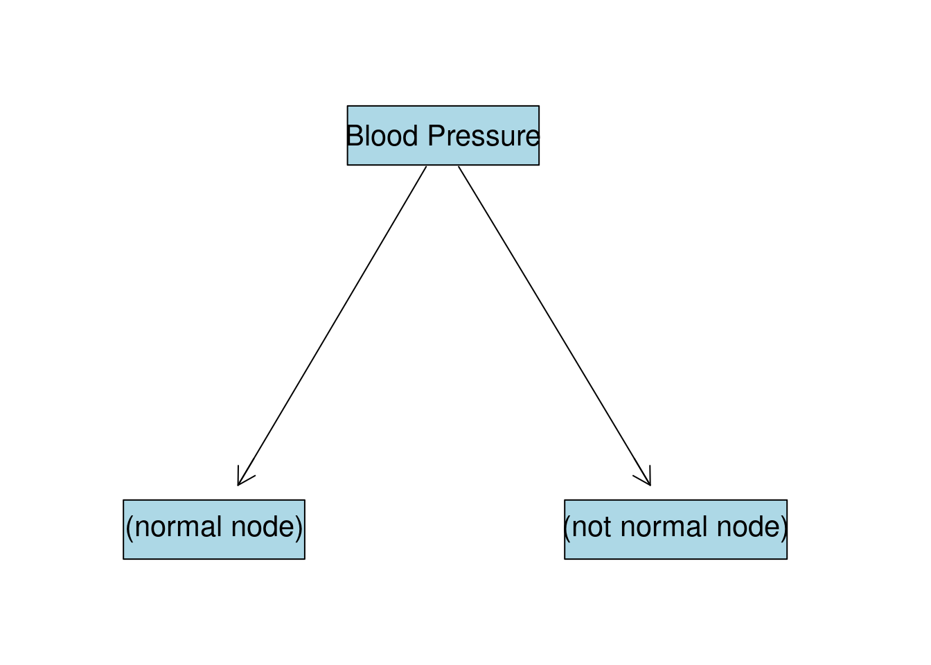
BP:normal Node
Continue to grow the tree down from the (normal node). We filter observations that have normal blood pressure:
train_df %>%
  filter(BP == "normal") %>%
  select(-BP) %>%
kable(format = "markdown")| Patient ID | Gender | BMI | Drug |
|---|---|---|---|
| p02 | M | not normal | Drug B |
| p06 | F | not normal | Drug B |
| p08 | F | not normal | Drug B |
| p12 | F | normal | Drug B |
| p13 | F | normal | Drug B |
| p15 | F | not normal | Drug B |
As we can see, there is no Drug A for this node and entropy is already 0. This node is going to be last for this branch with the drug B as an output with probability of 1. We can also think about this in a way that for all subjects with normal blood pressure drug B worked best.
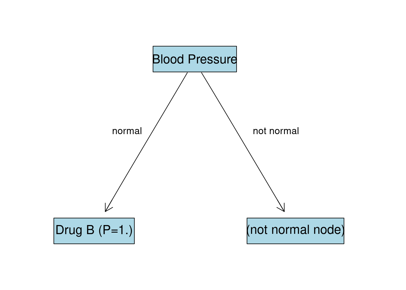
BP:not normal Node
Filter all the observations that have not normal blood pressure:
train_df %>%
  filter(BP == "not normal") %>%
  select(-BP) %>%
kable(format = "markdown")| Patient ID | Gender | BMI | Drug |
|---|---|---|---|
| p01 | M | not normal | Drug A |
| p03 | M | not normal | Drug A |
| p04 | M | normal | Drug A |
| p05 | M | not normal | Drug A |
| p07 | F | normal | Drug A |
| p09 | M | not normal | Drug A |
| p10 | M | normal | Drug A |
| p11 | F | not normal | Drug B |
| p14 | M | normal | Drug B |
Now we consider this set as “initial set”. The entropy of target distribution at this node is \(0.764\) (as we have already calculated it). At this node we have two features: Gender and BMI. We perform the same procedure to find the best splitting feature.
Gender
| Gender Label | Drug A | Drug B | P(A) | P(B) | Entropy | Weight | Weighted Entropy |
|---|---|---|---|---|---|---|---|
| M | 6 | 1 | \(\frac{6}{7}\) | \(\frac{1}{7}\) | 0.592 | \(\frac{7}{9}\) | 0.46 |
| F | 1 | 1 | \(\frac{1}{2}\) | \(\frac{1}{2}\) | 1 | \(\frac{2}{9}\) | 0.222 |
\[\text{IG} = 0.764 - (0.46 + 0.222) = 0.082\]
BMI
| BMI Label | Drug A | Drug B | P(A) | P(B) | Entropy | Weight | Weighted Entropy |
|---|---|---|---|---|---|---|---|
| normal | 4 | 1 | \(\frac{4}{5}\) | \(\frac{1}{5}\) | 0.722 | \(\frac{5}{9}\) | 0.401 |
| not normal | 3 | 1 | \(\frac{3}{4}\) | \(\frac{1}{4}\) | 0.811 | \(\frac{4}{9}\) | 0.361 |
\[\text{IG} = 0.764 - (0.401 + 0.361) = 0.002\]
Node Summary
Gender gives the highest IG after splitting the data. Now the tree will look like this:
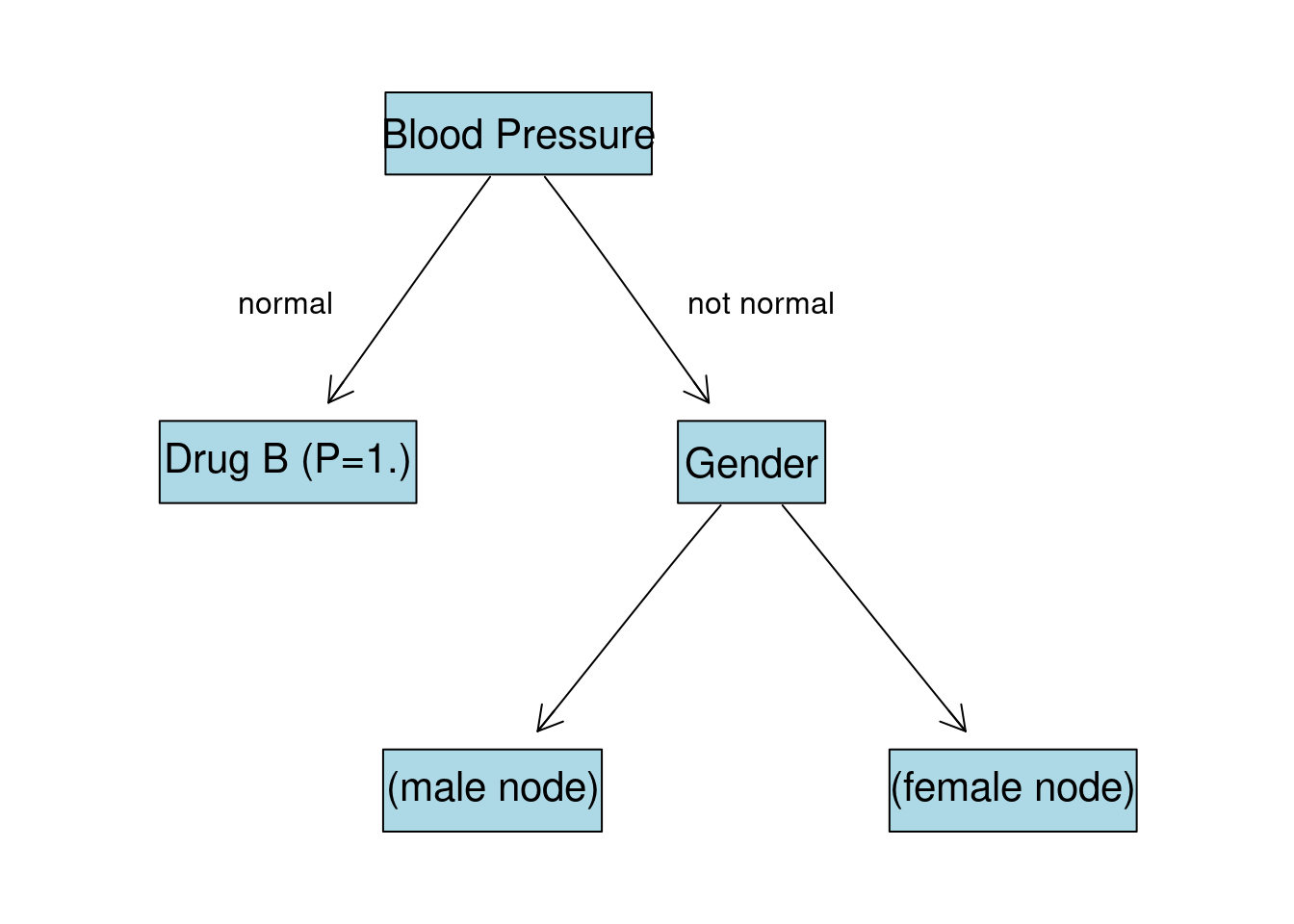
Gender:M Node
Now we filer the set so that we have only observations with BP:not normal and Gender:M:
train_df %>%
  filter(BP == "not normal" & Gender == "M") %>%
  select(-c(BP, Gender)) %>%
kable(format = "markdown")| Patient ID | BMI | Drug |
|---|---|---|
| p01 | not normal | Drug A |
| p03 | not normal | Drug A |
| p04 | normal | Drug A |
| p05 | not normal | Drug A |
| p09 | not normal | Drug A |
| p10 | normal | Drug A |
| p14 | normal | Drug B |
There is just one feature left BMI. Since we have no more features apart from this one we are going to “grow” last nodes with BMI:normal and BMI:not normal labels:
| BMI Label | Drug A | Drug B | P(A) | P(B) |
|---|---|---|---|---|
| normal | 2 | 1 | \(\frac{2}{3}\) | \(\frac{1}{3}\) |
| not normal | 4 | 0 | \(\frac{4}{4}\) | \(\frac{0}{4}\) |
For the BMI:normal node the predicted class is going to be Drug A, since its probability is higher. The same applies to BMI:not normal node.
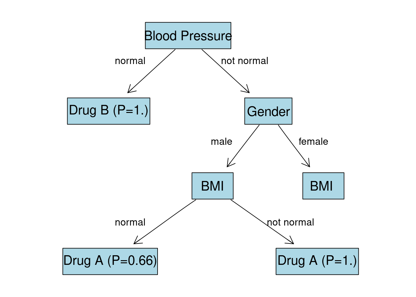
Gender:F Node
Now we filer the set so that we have only observations with BP:not normal and Gender:F:
train_df %>%
  filter(BP == "not normal" & Gender == "F") %>%
  select(-c(BP, Gender)) %>%
kable(format = "markdown") | Patient ID | BMI | Drug |
|---|---|---|
| p07 | normal | Drug A |
| p11 | not normal | Drug B |
We are left with just 1 observation in each node. Predicted class for node BMI:normal is going to be Drug A (\(P = 1.\)). Predicted class for node BMI:not normal is going to be Drug B (\(P = 1.\)).
Final Tree
Given all the calculations we visualize the final tree:
Code
node0 <- "Blood Pressure"
node1 <- "Drug B (P=1.)"
node2 <- "Gender"
node3 <- "BMI"
node4 <- "BMI "
node5 <- "Drug A (P=0.66)"
node6 <- "Drug A (P=1.)"
node7 <- "Drug A (P=1.) "
node8 <- "Drug B (P=1.) "
nodeNames <- c(node0, node1, node2, node3,
               node4, node5, node6, node7, node8)

# create new graph object
rEG <- new("graphNEL", nodes=nodeNames, edgemode="directed")
rEG <- addEdge(node0, node1, rEG)
rEG <- addEdge(node0, node2, rEG)
rEG <- addEdge(node2, node3, rEG)
rEG <- addEdge(node2, node4, rEG)
rEG <- addEdge(node3, node5, rEG)
rEG <- addEdge(node3, node6, rEG)
rEG <- addEdge(node4, node7, rEG)
rEG <- addEdge(node4, node8, rEG)

plot(rEG, attrs = at)
text(150, 300, "normal", col="black")
text(260, 300, "not normal", col="black")
text(200, 190, "male", col="black")
text(310, 190, "female", col="black")
text(100, 80, "normal", col="black")
text(230, 80, "not normal", col="black")
text(290, 80, "normal", col="black")
text(420, 80, "not normal", col="black")
Prediction
Let’s look at the 16th patient:
test_df %>%
kable(format = "markdown") | Patient ID | Gender | BMI | BP | Drug |
|---|---|---|---|---|
| p16 | M | not normal | not normal | ??? |
To make a prediction we just need to move top to bottom by the branches of our tree.
- Check
BP. SinceBP:not normal, go to the right branch. Gender:M=> left branch.BMI:not normal=> right branch.
The predicted value is going to be Drug A with a probability of \(1.0\).
Let Computer Do the Math
R
We can build a decision tree using rpart function (from rpart package) and plot it with the help of fancyRpartPlot function (from rattle package). Note, that R doesn’t require the categorical variables encoding since it can handle them by itself.
model_dt <- rpart(
  formula = Drug ~ Gender + BMI + BP,
  data = train_df,
  method = "class",
  minsplit = 1,
  minbucket = 1,
  parms = list(
    split = "information" # for Gini impurity change to split = "gini"
  )
)

#plot decision tree model
fancyRpartPlot(model_dt, caption = NULL, type=4)
Get a prediction for the 16th patient:
# return the class
predict(object = model_dt, newdata = test_df, type = "class")
##      1
## Drug A
## Levels: Drug A Drug B

# return the probability of each class
predict(object = model_dt, newdata = test_df, type = "prob")
##      Drug A    Drug B
## 1 0.8571429 0.1428571
Note that since R didn’t split Gender:M node by BMI the probabilities are quite different that we expected but it doesn’t effect the predicted class.
Python
Unlike R, Python doesn’t allow categorical input variables, so we need to encode them:
patients_df = pd.read_csv("DecisionTree_SampleData.csv")
# drop id column
patients_df.drop('Patient ID', axis=1, inplace=True)

# convert to dummy variables
patients_df_labeled = pd.get_dummies(patients_df)
columns_to_drop = ['Gender_F', 'BMI_not normal', 'BP_not normal', 'Drug_???', 'Drug_Drug B']
patients_df_labeled.drop(
    columns_to_drop,
    axis=1,
    inplace=True)
unknown_drug = patients_df_labeled.iloc[15, :]
patients_df_labeled.drop(15, axis=0, inplace=True) # unknow drug row
patients_df_labeled.head().to_html(classes='table table-striped')| Gender_M | BMI_normal | BP_normal | Drug_Drug A | |
|---|---|---|---|---|
| 0 | 1 | 0 | 0 | 1 |
| 1 | 1 | 0 | 1 | 0 |
| 2 | 1 | 0 | 0 | 1 |
| 3 | 1 | 1 | 0 | 1 |
| 4 | 1 | 0 | 0 | 1 |
For example Gender_M:1 means that subject is Male and Gender_M:0 means that subject is female.
To build a decision tree model we can use a DecisionTreeClassifier function from sklearn.tree module.
# split the data
X = patients_df_labeled.drop('Drug_Drug A', axis=1)
y = patients_df_labeled['Drug_Drug A']

# fit the decision tree model
model = tree.DecisionTreeClassifier(
  criterion='entropy' # for Gini impurity change to criterion="gini"
)
model.fit(X, y)
## DecisionTreeClassifier(criterion='entropy')
# plot the tree
plt.figure(figsize=(10,10))
tree.plot_tree(
model, filled=True, rounded=True,
feature_names=X.columns.tolist(), proportion=False,
class_names=['Drug B', 'Drug A']
)
plt.show()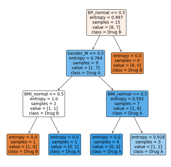
Get a prediction for the 16th patient:
unknown_drug = pd.DataFrame(unknown_drug).T
unknown_drug.drop(['Drug_Drug A'], axis=1, inplace=True)

# return the class
model.predict(unknown_drug)
## array([1], dtype=uint8)
# return the probability of each class
model.predict_proba(unknown_drug)
## array([[0., 1.]])Numerical Explanatory Variables
In our sample data set, we had only categorical variables (with 2 labels each). But what would the model do, if we had numerical value as an input?
Let’s look again on the Python decision tree and its decision node conditions, for example, Gender_M <= 0.5. Where does 0.5 come from? The answer overlaps with the answer on how the model handles numerical input values.
Recall the Gender_M column we created for the Python train set. It consisted of two numerical values (0 and 1). What the model does is filter the data by the average value among these two numbers. Average value was: \(\frac{0+1}{2}=0.5\). Now model has two sets of data: one set that matches the condition Gender_M <= 0.5 (Gender is female) and the other set that doesn’t (Gender is male).
Imagine that we have added a third category Non-binary to the Gender feature. First, we would encode the values and create a new column Gender_encoded, which would have three numerical values (0, 1 and 2). Say, Non-binary = 0, Male = 1, Female = 2. Now model would have two conditions for filtering the data:
Gender_encoded <= 0.5(Genderis non-binary)Gender_encoded <= 1.5(Genderis non-binary OR male)
In a general way, we can say that if we have a numerical feature, the algorithm will convert it to “categorical” by choosing the average value as a threshold between actual input values:
- filter 1: feature <= threshold
- filter 2: feature > threshold
For example:
| id | blood_pressure | drug |
|---|---|---|
| p01 | 100 | A |
| p02 | 120 | B |
| p03 | 150 | B |
| p03 | 200 | B |
Threshold values are: 110 \(\left( \frac{100+120}{2} \right)\), 135 \(\left( \frac{120+150}{2} \right)\), 175 \(\left( \frac{150+200}{2} \right)\).
Other Splitting Metrics
Gini Impurity
As told before, for classification problems one can also use Gini impurity as a way to find the best splitting feature. The idea stays the same, but the only difference is that instead of the Entropy formula we are using the Gini formula:
\[G(X) = 1 - \sum_{i=1}^{n} p(x_i)^2\] After calculating the Gini impurity value for each feature, we would calculate the gain and choose the feature that provides the highest gain.
\[\scriptsize \text{Gain} = \text{Gini impurity before the split} - \text{Weighted Gini impurity after the split}\]
Variance Reduction
If we are dealing with the regression problem (predicting numerical variable, rather than a class) we would use the variance reduction. Instead of calculating the probabilities of the target variable we calculate its variance:
\[Var(x) = \frac{\sum_{i=1}^n(x_i- \bar x)^2}{n-1}\] And in the same way we are looking for a variable that has the highest variance reduction, or in other words variance in the target variable becomes lower after the split.
\[\scriptsize \text{Variance Reduction} = \text{Variance before the split} - \text{Weighted variance after the split}\]
Summary
We have looked at the example of the CART model for the binary classification problem. It is a relatively simple algorithm that doesn’t require much feature engineering. With the small data set and lots of free time, one can even build a model with “pen and paper”. Compared to other ML algorithms, CART can be considered as a “weak learner” due to the overfitting issue. However, they are often used as a base estimator in more complex bagging and boosting models (for example, Random Forest algorithm). Additionally, CART can help with the hidden data patterns, since they can be visualized.