Null Hypothesis Significance Testing, part 2
Inference for a population proportion: binomial test, χ$^2$ test.
Cover image credit: TheDigitalArtist from Pixabay
Table of contents
# r import
library(tidyverse)
library(knitr)
library(reticulate)
library(corrplot)

options(digits = 4)
use_python("/home/ruslan/anaconda3/bin/python3.7")
# python import
import pandas as pd
from scipy import stats# custom functions
nhst_result <- function(pval, alpha){
if(pval < alpha) {
print(paste0("p-value is less than alpha (",
alpha, "). Reject the null hypothesis."))
} else {print(paste0("p-value is greater than alpha (",
alpha, "). Fail to reject the null hypothesis."))}
}Introduction
In the previous part1 we’ve looked and the basic idea of the statistical testing and the inference for a population mean (\(\mu\)). Here we are going to look at the inference for a population proportion (\(p\) or \(\pi\)).
Data Set
We are going to look at the Student Alcohol Consumption dataset (Math sample) from Kaggle2.
Context of the problem: The data were obtained in a survey of student’s math and Portuguese language courses in secondary school. It contains a lot of interesting social, gender and study information about students.
Data set consist of 30 explanatory variables such as weekly study time or parents education level and three target variables which show the final grade for a math exam:
G1- first period grade (numeric: from 0 to 20)G2- second period grade (numeric: from 0 to 20)G3- final grade (numeric: from 0 to 20, output target)
Original paper: P. Cortez and A. Silva. Using Data Mining to Predict Secondary School Student Performance. In A. Brito and J. Teixeira Eds., Proceedings of 5th FUture BUsiness TEChnology Conference (FUBUTEC 2008) pp. 5-12, Porto, Portugal, April, 2008, EUROSIS, ISBN 978-9077381-39-73.
students_data <- read_csv("data/student-mat.csv")
sample_n(students_data, 5) %>% kable()| school | sex | age | address | famsize | Pstatus | Medu | Fedu | Mjob | Fjob | reason | guardian | traveltime | studytime | failures | schoolsup | famsup | paid | activities | nursery | higher | internet | romantic | famrel | freetime | goout | Dalc | Walc | health | absences | G1 | G2 | G3 |
|---|---|---|---|---|---|---|---|---|---|---|---|---|---|---|---|---|---|---|---|---|---|---|---|---|---|---|---|---|---|---|---|---|
| GP | F | 15 | U | GT3 | T | 1 | 1 | other | other | home | father | 1 | 2 | 0 | no | yes | no | yes | no | yes | yes | no | 4 | 3 | 2 | 2 | 3 | 4 | 2 | 9 | 10 | 10 |
| GP | M | 20 | U | GT3 | A | 3 | 2 | services | other | course | other | 1 | 1 | 0 | no | no | no | yes | yes | yes | no | no | 5 | 5 | 3 | 1 | 1 | 5 | 0 | 17 | 18 | 18 |
| GP | F | 19 | U | GT3 | T | 2 | 1 | at_home | other | other | other | 3 | 2 | 0 | no | yes | no | no | yes | no | yes | yes | 3 | 4 | 1 | 1 | 1 | 2 | 20 | 14 | 12 | 13 |
| GP | M | 16 | U | GT3 | T | 4 | 4 | services | services | course | mother | 1 | 1 | 0 | no | no | no | yes | yes | yes | yes | no | 5 | 3 | 2 | 1 | 2 | 5 | 0 | 13 | 12 | 12 |
| GP | F | 17 | U | GT3 | T | 4 | 4 | other | teacher | course | mother | 1 | 1 | 0 | yes | yes | no | no | yes | yes | no | yes | 4 | 2 | 1 | 1 | 1 | 4 | 0 | 11 | 11 | 12 |
Inference for a Proportion
We have already discussed how you can run a test for a continuous random variable (such as weight, distance, glucose level, etc.). But what if your variable of interest is not continuous but rather discreet (for example, ratio of success for a new drug, the exam score, etc.)?
Single Proportion
Imagine that previous research suggests that on average 60% of students pass the final math exam. Can we say that this rate became larger after the new data came in?
- \(H_0\): Student success rate for a final math exam is 60%, \(\pi=0.6\).
- \(H_A\): Student success rate for a final math exam is greater than 60%, \(\pi>0.6\)
- \(\alpha = 0.05\)
According to the paper, exam is passed is the score is greater than 9, so we are going to create a new variable with binary outcome pass/fail:
students_data <- students_data %>%
    mutate(final_score = if_else(G3 > 9, "pass", "fail"))

p_sample <- mean(students_data$final_score == "pass")
print(paste0("p = ", round(p_sample, 4)))
## [1] "p = 0.6709"Code
ggplot(data = students_data, aes(x = final_score, fill = final_score)) +
    geom_bar() +
    labs(title = "Final Math Exam Results",
         x = "Result")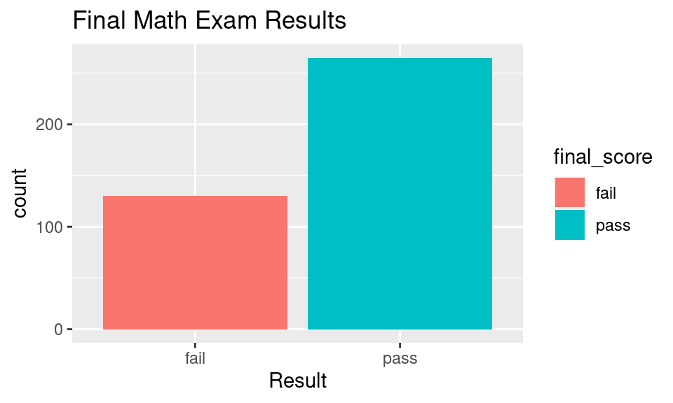
Now, the variable final_score is actually falling under Binomial distribution4. We have (kind of) looked already at how to deal with binomial distributed variables under the null hypothesis testing framework in this intuitive example5, but let’s dig into more details.
We are going to use the binomial test6 in order to find the p-value.
The idea stays the same, we want to know the probability of observing data as extreme as we got during the experiment (\(p=0.67\)) under the assumption that the null hypothesis is true (\(\pi=0.6\)). The Binomial distribution is defined as:
\[P(X=k) = C_n^k p^k (1-p)^{n-k}\]
- \(n\) - number of trials;
- \(p\) - success probability for each trial;
- \(k\) - number of successes.
Let’s draw the null distribution:
Code
n <- dim(students_data)[1] # total number of strudents
p_null <- 0.6
n_passed <- sum(students_data$final_score == "pass")

x <- 200:275
b_dist <- dbinom(x, p = p_null, size = n)

fill <- rep("red", length(x))
fill[x >= n_passed] <- "lightblue"

ggplot(data = students_data, aes(x = final_score, fill = final_score)) +
    geom_bar() +
    labs(title = "Final Math Exam Results",
         x = "Result")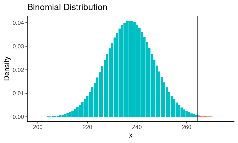
We would expect 237 students of 395 to pass the math exam under the assumption that the null hypothesis is true (\(n \times \pi = 395 \times 0.6 = 237\)). That is the expected value of a null distribution. We have observed 265 students who have passed the test. So now the p-value is the sum of probabilities for \(x\) greater or equal to 265:
\[\scriptsize \text{p-value} = P(X=237) + P(X=238) + ... + P(X=395)\]
\[\scriptsize P(X=237) = C_{395}^{237} \times 0.6^{237} \times (1-0.6)^{395-237}\]
\[\scriptsize P(X=238) = C_{395}^{238} \times 0.6^{238} \times (1-0.6)^{395-238}\]
\[...\]
\[\scriptsize P(X=395) = C_{395}^{395} \times 0.6^{395} \times (1-0.6)^{395-395}\]
As we can see, that is a lot of calculations to do by hand. There is a way to use Normal approximation7 which would allow to calculate the p-value with less effort, but we are going to rely on R:
pval <- 1 - pbinom(q = n_passed, p = p_null, size = n)
print(paste0("p-value is: ", round(pval, 3)))
## [1] "p-value is: 0.002"alpha <- 0.05
nhst_result(pval, alpha)## [1] "p-value is less than alpha (0.05). Reject the null hypothesis."And of course, there are implementations for a binomial test that allow skipping most of the calculations:
R
Built-in binom.test function:
binom.test(n_passed, n, p_null, "greater")##
## Exact binomial test
##
## data: n_passed and n
## number of successes = 265, number of trials = 395, p-value = 0.002
## alternative hypothesis: true probability of success is greater than 0.6
## 95 percent confidence interval:
## 0.6299 1.0000
## sample estimates:
## probability of success
## 0.6709Python
binom_test function from scipy.stats module:
students_data = pd.read_csv("data/student-mat.csv")
students_data["final_score"] = students_data["G3"].apply(lambda x: "pass" if x>9 else "fail")

p_null = 0.6
n = students_data.shape[0]
n_passed = sum(students_data["final_score"] == "pass")

p_val = stats.binom_test(x=n_passed, n=n, p=p_null, alternative="greater")
print(f"p-value: {p_val: .4f}")
## p-value: 0.0022Multiple Proportions
Now say we want to compare proportion for multiple groups rather than just one. For this purpose one can use \(\chi^2\) test for independence. In general form, under the chi-square test we have following hypotheses:
- \(H_0\): There is no association between groups.
- \(H_A\): There is an association between the groups (one-sided test).
Conditions for \(\chi^2\) test:
- Independence
- Sample size (each “cell” must have at least 5 expected cases)
Test statistic \(\chi^2\) (which is following \(\chi^2\) distribution8) can be found as:
\[\chi^2 = \sum_{i=1}^k \frac{(O-E)^2}{E}\]
- \(O\): observed data in a “cell”
- \(E\): expected data of a “cell”
- \(k\): number of “cells”
Example
Does alcohol consumption level on weekends affect the student study results?
- \(H_0\): exam results and alcohol consumption are independent.
- \(H_A\): exam results and alcohol consumption are dependent (results scores vary by alcohol consumption).
- \(\alpha = 0.05\)
There are 5 levels of alcohol consumption (from 1 - very low to 5 - very high). First, we can take a look at the cross tab to see the number of observations in each group:
ct <- table(students_data$final_score, students_data$Walc)
ct %>% kable()| 1 | 2 | 3 | 4 | 5 | |
|---|---|---|---|---|---|
| fail | 50 | 25 | 25 | 20 | 10 |
| pass | 101 | 60 | 55 | 31 | 18 |
Each cell has more than 5 observations, so we can say that the sample size condition is met.
We are going to rewrite the previous cross table in the following way:
| Weekend alcohol consumption level | 1 | 2 | 3 | 4 | 5 | Total |
|---|---|---|---|---|---|---|
| Failed | 50 (50) | 25 (28) | 25 (26) | 20 (17) | 10 (9) | 130 |
| Passed | 101 (101) | 60 (57) | 55 (54) | 31 (34) | 18 (19) | 265 |
| Total | 151 | 85 | 80 | 51 | 28 | 395 |
Numbers in parentheses is the expected number of observations for each cell. Assuming that there is no association between the groups we expect 67.09% of students to pass the exam (\(p =\frac{\text{total passed}}{\text{total}} = \frac{265}{395}=0.6709\)) in each group. Let’s take a look at a 1 level of alcohol consumption. Given that assumption we expect to observe 101 students who passed the exam (\(\text{total for 1 level} \times p\) \(= 151 \times 0.6709 = 101\)). Hence we expect 50 students to fail the exam (\(151-101 = 50\)).
For the second (2) level of alcohol consumption we expect to observe 57 students who passed the exam (\(\text{total for 2 level} \times p = 85 \times 0.6709 = 57\)) and 28 who failed (\(85-57 = 28\)). And so on for each group. After we found the expected values for each cell we can calculate the \(\chi^2\) value:
\[\scriptsize \chi^2 = \frac{(50-50)^2}{50} + \frac{(25-28)^2}{28} + ... + \frac{(18-19)^2}{19}\]
This also may be a tough task to calculate by hand that’s why we usually rely on software.
R
Built-in chisq.test function:
results <- chisq.test(ct, correct = FALSE)
results
##
## Pearson's Chi-squared test
##
## data: ct
## X-squared = 1.6, df = 4, p-value = 0.8Python
chi2_contingency function from scipy.stats module:
ct = pd.crosstab(students_data.final_score, students_data.Walc).to_numpy()
chisq_stat, p_val, dof, expctd = stats.chi2_contingency(ct, correction=False)
print(f"Calculated test statistic: {chisq_stat: .4f}\np-value: {p_val: .4f}")
## Calculated test statistic: 1.5919
## p-value: 0.8102
A couple of notes:
- Degrees of freedom can be found as \(df=(C-1)(R-1)\), where \(C\) - number of columns, \(R\) - number of rows.
correctionargument in chi-square test function is used for the Yates’s correction for continuity9.
Code
x <- seq(0,10,0.1)
df <- 4
chisq_dist <- dchisq(x, df)
chi_sq <- results$statistic

ggplot() +
  geom_line(
    mapping = aes(x = x, y = chisq_dist),
    color = "black", size = 1.5) +
  geom_vline(xintercept = chi_sq) +
  geom_area(
    mapping = aes(x = x[x >= chi_sq], y = chisq_dist[x >= chi_sq]),
    fill="red", alpha=0.6) +
  labs(title = "Chi-square Distribution",
       y = "Density") +
  theme_classic()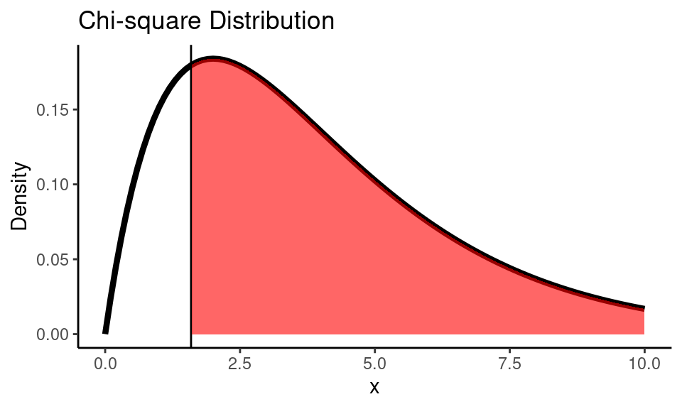
R also lets us explore the expected and observed count
results$observed %>% kable()| 1 | 2 | 3 | 4 | 5 | |
|---|---|---|---|---|---|
| fail | 50 | 25 | 25 | 20 | 10 |
| pass | 101 | 60 | 55 | 31 | 18 |
results$expected %>% kable()| 1 | 2 | 3 | 4 | 5 | |
|---|---|---|---|---|---|
| fail | 49.7 | 27.97 | 26.33 | 16.78 | 9.215 |
| pass | 101.3 | 57.03 | 53.67 | 34.22 | 18.785 |
Also, we can check the residual values of each cell, that are defined as:
\[r = \frac{O-E}{\sqrt{E}}\]
residuals_table <- results$residuals
kable(residuals_table)| 1 | 2 | 3 | 4 | 5 | |
|---|---|---|---|---|---|
| fail | 0.0431 | -0.5624 | -0.2590 | 0.7848 | 0.2585 |
| pass | -0.0302 | 0.3939 | 0.1814 | -0.5497 | -0.1811 |
corrplot(residuals_table)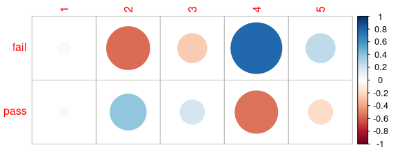
High residual values mean that this cell has the highest influence on a \(\chi^2\) score. Another approach would be to find the percentage of contribution using the formula:
\[\text{Cell Contribution} = \frac{r}{\chi^2} \times 100\%\]
contrib_table <- 100 * residuals_table^2 / results$statistic
kable(contrib_table)| 1 | 2 | 3 | 4 | 5 | |
|---|---|---|---|---|---|
| fail | 0.1167 | 19.870 | 4.215 | 38.69 | 4.199 |
| pass | 0.0572 | 9.748 | 2.068 | 18.98 | 2.060 |
As we can see, the pairs of fail & 2, fail & 4 and pass & 4 have the highest percentage of contribution (or in other words, there is some association).
Summary
This was a brief overview of how we can perform hypothesis testing when we deal with discrete variables. In the next (and I hope the final) part I will finally introduce a concept of test power and effect size and discuss why p-value alone is not sufficient for decision making.
References
Cortez, Paulo & Silva, Alice. (2008). Using data mining to predict secondary school student performance. EUROSIS.↩︎