Null Hypothesis Significance Testing, part 3
Power of the Test, Sample Size and Effect Size
Cover image credit: Pixabay from Pexels
Table of contents
# r import
library(tidyverse)
library(knitr)
library(reticulate)
library(pwr)
library(metRology)
library(effsize)

options(digits = 4)
use_python("/home/ruslan/anaconda3/bin/python3.7")
# python import
import pandas as pd
from statsmodels.stats import power# custom functions
nhst_result <- function(pval, alpha){
if(pval < alpha) {
print(paste0("p-value is less than alpha (",
alpha, "). Reject the null hypothesis."))
} else {print(paste0("p-value is greater than alpha (",
alpha, "). Fail to reject the null hypothesis."))}
}Introduction
In the two previous parts1\(^,\)2 we have reviewed the idea of inference for a population mean and proportion under the null hypothesis significance testing framework. The idea is pretty simple - find the probability of the occurrence of experimental data using the assumption that null hypothesis is true (p-value), if it’s lower than significance level (\(\alpha\)), then reject the null hypothesis in favor of an alternative hypothesis. \(\alpha\) is the probability of rejecting \(H_0\) when, in fact, it is true and we, obviously, want to keep it low. But as told before there might be another place for an error, and that is failing to reject the \(H_0\) when in fact it is false. This is called Type II error and the probability of this is denoted as \(\beta\).
| \(H_0\) is true | \(H_0\) is false | |
|---|---|---|
| Failed to reject \(H_0\) | No Error (\(1-\alpha\)) | Type II Error (\(\beta\)) |
| Reject \(H_0\) in favor of \(H_A\) | Type I Error (\(\alpha\)) | No Error (\(1-\beta\)) |
Power of the Test
The value of \(1 - \beta\) is called the power of a test and we also want the power to be high (or the \(\beta\) to be small). Commonly used value for the power is 80% (\(\beta = 0.2\)).
Let’s imagine the following example. You are developing a new drug that helps people with insomnia. Study shows that on average people with insomnia sleep on average 4 hours a day. You would like to check whether your drug helps to increase the sleep time.
- \(H_0\): a new drug has no effect on a sleep time for people with insomnia; \(\mu = 4\)
- \(H_A\): a new drug increases the sleep duration; \(\mu > 4\)
- \(\alpha = 0.05\)
For simplicity, let’s assume that \(n\) is greater than 30 and \(\sigma\) is known and equal to 1. Under this assumptions we could use the \(Z\) statistic to find the p-value:
\[Z = \frac{\bar{X} - \mu}{SE}\]
\[SE = \frac{\sigma}{\sqrt{n}}\] We would reject the null hypothesis if \(Z \geq Z_{1-\alpha}\). We want to observe the difference of at least half on hour (0.5) in increase of a sleep duration, meaning that \(\mu_A=4+0.5 = 4.5\) hours. What would be the power of the test if we collected data from 15 patients?
Code
mu_null <- 4
mu_alt <- 4.5
sd <- 1
n <- 15
se <- sd/sqrt(n)
Z_crit <- qnorm(0.95) * se + mu_null
x <- seq(2,7,0.01)
null_dist <- dnorm(x = x, mean = mu_null, sd = se)
observed_dist <- dnorm(x = x, mean = mu_alt, sd = se)

ggplot() +
  geom_line(
    mapping = aes(x = x, y = null_dist),
    color = "black", size = 1) +
  geom_line(
    mapping = aes(x = x, y = observed_dist),
    color = "grey", size = 1) +
  geom_vline(xintercept = mean(Z_crit), color = "red", linetype = "dashed") +
  geom_area(mapping = aes(x = x[x >= Z_crit], y = observed_dist[x >= Z_crit]),
    fill = "blue", alpha = 0.5) +
  geom_area(mapping = aes(x = x[x >= Z_crit], y = null_dist[x >= Z_crit]),
    fill = "red", alpha = 0.5) +
  annotate(
    geom = "curve", x = 2.5, y = 0.5, xend = 3.5, yend = null_dist[x == 3.5],
    curvature = .3, arrow = arrow(length = unit(2, "mm"))) +
  annotate(geom = "text", x = 2, y = 0.55, label = "Null Distribution", hjust = "left") +
  annotate(
    geom = "curve", x = 3.2, y = 1, xend = 4.2, yend = observed_dist[x == 4.2],
    curvature = .3, arrow = arrow(length = unit(2, "mm"))) +
  annotate(geom = "text", x = 3.2, y = 1.05, label = "Alternative Distribution", hjust = "right") +
  annotate(
    geom = "curve", x = 5.5, y = 0.2, xend = 4.5, yend = 0.05,
    curvature = .3, arrow = arrow(length = unit(2, "mm"))) +
  annotate(geom = "text", x = 5.55, y = 0.2, label = "alpha; rejection region", hjust = "left") +
  annotate(
    geom = "curve", x = 5.5, y = 0.8, xend = 4.8, yend = 0.5,
    curvature = .3, arrow = arrow(length = unit(2, "mm"))) +
  annotate(geom = "text", x = 5.55, y = 0.8, label = "Power", hjust = "left") +
  annotate(
    geom = "curve", x = 5.5, y = 1.2, xend = Z_crit, yend = 1.2,
    curvature = .3, arrow = arrow(length = unit(2, "mm"))) +
  annotate(geom = "text", x = 5.55, y = 1.2, label = "Z critical", hjust = "left") +
  labs(y = "Density") +
  theme_classic()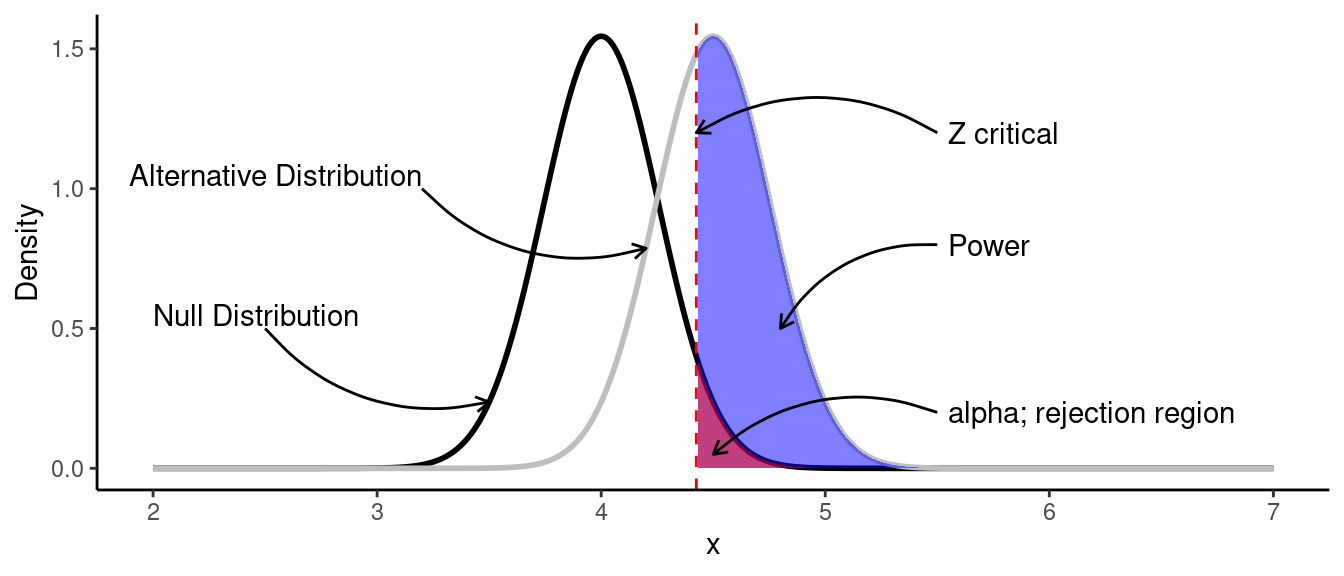
Let’s look deeper at this plot:
- Black line is the null distribution with the parameters \(\mu_0=4\) and \(\sigma=0.5\).
- Gray line is the distribution of the data we would like to observe (alternative distribution) with the parameters \(\mu_A=4.5\) and \(\sigma=0.5\).
- Red area is the rejection area, which is above the .95 quantile of the null distribution. We would reject the null hypothesis if the calculated \(Z\) statistic is greater \(Z\) critical.
- Blue area is the power of a test. It’s the probability of rejecting the null hypothesis when it is false.
In such case we could find the power by finding the area under the curve of the observed data:
\[\scriptsize \text{Power} = P \left( X \geq Z_{crit} \mid \mu = 4.5, \sigma = \frac{1}{\sqrt{15}} \right)\]
Critical value of \(Z\) can be found as:
\[\scriptsize Z_{crit} = Q_{0.95} \times \frac{\sigma}{\sqrt{n}} + \mu_0\]
Where \(Q_{0.95}\) is the 0.85 quantile of the standard normal distribution.
\[\scriptsize Z_{crit} = 1.645 \times \frac{1}{\sqrt{15}} + 4 = 4.425\]
Now, the power of the test can be find using R (instead of calculating the integral):
Z_crit <- qnorm(0.95) * se + mu_null
power <- pnorm(Z_crit, mean = mu_alt, sd = se, lower.tail = FALSE)
print(paste0("Power of the test is: ", round(power, 3)))
## [1] "Power of the test is: 0.615"As we can see, the highest possible power that can be achieved is 61.5%, which is lower than 80%. We could also see that power is dependent on a sample size \(n\) and the standard deviation \(\sigma\). We don’t really have control over \(\sigma\), but we have control over the sample size. If we increase the sample size from 15 to 50 observations, the standard error will decrease and hence, the power will increase:
Code
mu_null <- 4
mu_alt <- 4.5
sd <- 1
n <- 50
se <- sd/sqrt(n)
Z_crit <- qnorm(0.95) * se + mu_null
x <- seq(2,7,0.005)
null_dist <- dnorm(x = x, mean = mu_null, sd = se)
observed_dist <- dnorm(x = x, mean = mu_alt, sd = se)

ggplot() +
  geom_line(
    mapping = aes(x = x, y = null_dist),
    color = "black", size = 1) +
  geom_line(
    mapping = aes(x = x, y = observed_dist),
    color = "grey", size = 1) +
  geom_vline(xintercept = mean(Z_crit), color = "red", linetype = "dashed") +
  geom_area(mapping = aes(x = x[x >= Z_crit], y = observed_dist[x >= Z_crit]),
    fill = "blue", alpha = 0.5) +
  geom_area(mapping = aes(x = x[x >= Z_crit], y = null_dist[x >= Z_crit]),
    fill = "red", alpha = 0.5) +
  labs(y = "Density") +
  theme_classic()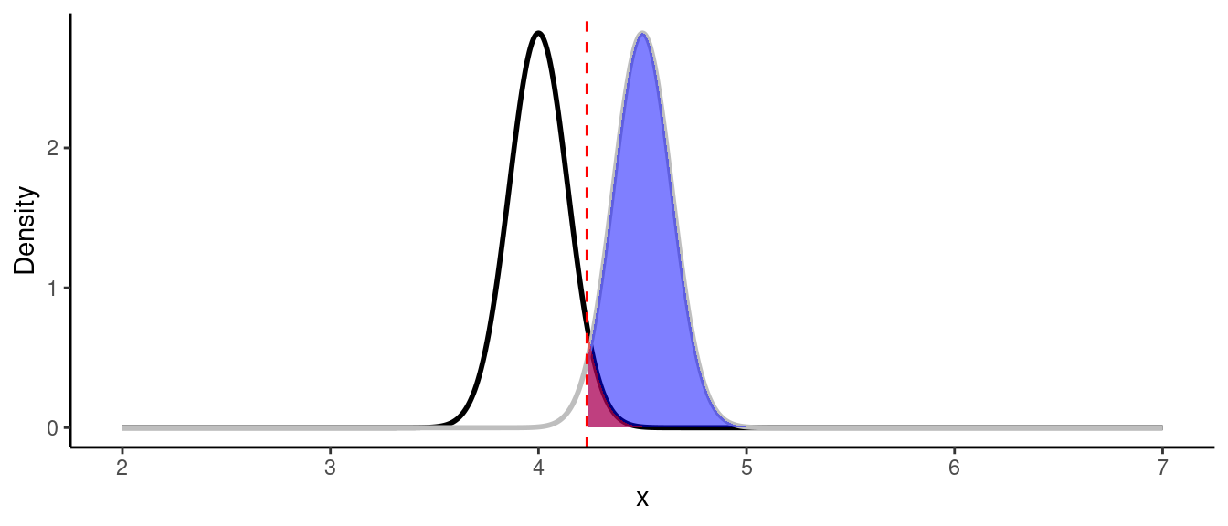
Z_crit <- qnorm(0.95) * se + mu_null
power <- pnorm(Z_crit, mean = mu_alt, sd = se, lower.tail = FALSE)
print(paste0("Power of the test is: ", round(power, 3)))
## [1] "Power of the test is: 0.971"In practice you want to know what sample size do you need to get be able to observe the difference with the desired levels of $ and \(\beta\) before the experiment.
Since most of the times we don’t know the population standard deviation \(\sigma\) we use \(t\) distribution. As you could see with the \(Z\) test example, calculations usually are a bit complicated to do by hand, that’s why we rely on R/Python.
For example, what is the minimum sample size we would require in order to observe the increase of a sleep duration of 0.5 hour with \(\alpha = 0.05\) and \(\beta = 0.2\)?
R
The power.t.test function from pwr package in R is pretty simple. There are 4 parameters - sample size n, standard deviation sd, delta d (which is the desired difference that you want to observe) and power power. In order to find the desired value for one of four values, enter the rest three values.
power.t.test(sd = sd, d = 0.5, power = 0.8,
             type = "one.sample", alternative = "one.sided")
##
## One-sample t test power calculation
##
## n = 26.14
## delta = 0.5
## sd = 1
## sig.level = 0.05
## power = 0.8
## alternative = one.sidedPython
tt_solve_power from statsmodels.stats.power works in the same way. The only difference that instead of delta you need to unout the value of effect_size which is the mean divided by the standard deviation for the one-sample test.
n = power.tt_solve_power(effect_size=0.5, power=0.8,
                         alpha=0.05, alternative='larger')
print(f'Required sample size: {n: .2f}')
## Required sample size: 26.14
As we can see, the minimum sample size is 27 observations.
Let’s find out how sample size changes the power in the previous example settings:
n <- 1:100
results <- power.t.test(n = n, sd = sd, d = 0.5,
                        type = "one.sample", alternative = "one.sided")
power_arr <- results$power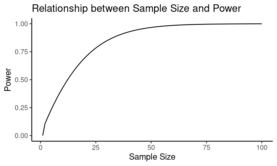
As we can see, the power of a test increases as the sample size increases.
Effect Size
Usually for calculating the sample size and power of the two sample test, one uses effect size instead of the absolute difference between null and alternative values. The most frequently used type of an effect size is Cohen’s \(d\), which can be defined asthe difference between two means divided by a standard deviation for the data:
\[\scriptsize d = \frac{\bar{x_1} - \bar{x_2}}{s_{pooled}} = \frac{\mu_1 - \mu_2}{s_{pooled}}\]
\(s_{pooled}\) - pooled standard deviation.
\[\scriptsize s_{pooled} = \sqrt{\frac{(n_1 -1)s_1^2 + (n_2 - 1)s_2^2}{n_1 + n_2 -2}}\]
The magnitude of Cohen’s \(d\) are usually referred as:
| Effect size | d |
|---|---|
| Very small | 0.01 |
| Small | 0.20 |
| Medium | 0.50 |
| Large | 0.80 |
| Very large | 1.20 |
| Huge | 2.0 |
For example, what sample size do you need to observe the large effect size (in any direction) when comparing two means (\(\alpha=0.05\), \(\beta=0.2\))?
R
In R you just have to change the parameter type to two.sample for dealing with two-sample \(t\) test.
power.t.test(delta = 0.8, power = 0.8, sig.level = 0.05,
             alternative = "two.sided", type = "two.sample")
##
## Two-sample t test power calculation
##
## n = 25.52
## delta = 0.8
## sd = 1
## sig.level = 0.05
## power = 0.8
## alternative = two.sided
##
## NOTE: n is number in *each* groupNote, that you cannot pass the effect size inside the function, but you can pass the delta (\(\mu_1-\mu_2\)) and sd (standard deviation) that will lead to desired effect size.
pwr package can be found at CRAN3.Python
tt_ind_solve_power function from statsmodels.stats.power deals with solving for any one parameter of the power of a two sample t-test.
n = power.tt_ind_solve_power(effect_size=0.8, power=0.8,
                             alpha=0.05, alternative='two-sided')
print(f'Required sample size: {n: .2f}')
## Required sample size: 25.52Why is it Important
The question you might ask is why would we care about the effect size if results show significant statistical difference? The problem is than even if the p-value < \(\alpha\), the observed effect size might be small (\(d< 0.5\)).
With a sufficiently large sample, a statistical test will almost always demonstrate a significant difference, unless there is no effect whatsoever, that is, when the effect size is exactly zero; yet very small differences, even if significant, are often meaningless. Thus, reporting only the significant p-value for an analysis is not adequate for readers to fully understand the results.4
Consider a following example. You are developing the drug for people with diabetes to reduce blood sugar level. You have a treatment (drug) and control (placebo) groups with 150 subjects in each.
- \(H_0\): new drug doesn’t reduce the sugar level (\(\mu_t=\mu_c\));
- \(H_A\): new drug reduces the sugar level (\(\mu_t < \mu_c\));
- \(\alpha = 0.05\)
Case #1
set.seed(1)
sample_control <- rnorm(n = 150, mean = 150, sd = 20)
sample_treatment <- rnorm(n = 150, mean = 145, sd = 20)
ttest_results <- t.test(sample_treatment, sample_control,
                        alternative = "less")
ttest_results
##
## Welch Two Sample t-test
##
## data: sample_treatment and sample_control
## t = -2, df = 294, p-value = 0.02
## alternative hypothesis: true difference in means is less than 0
## 95 percent confidence interval:
## -Inf -0.849
## sample estimates:
## mean of x mean of y
## 145.9 150.4Code
ggplot() +
  geom_histogram(aes(sample_control, fill = "blue"), bins = 10,
                 color = "black", alpha = 0.5) +
  geom_histogram(aes(sample_treatment, fill = "orange", ), bins = 10,
                 color = "black", alpha = 0.5) +
  labs(title = "Sample Distribution",
       y = "Count",
       x = "Sugar Level") +
  scale_fill_manual(name = "Group", values = c("blue", "orange"),
                    labels = c("Control", "Treatment")) +
  theme_classic()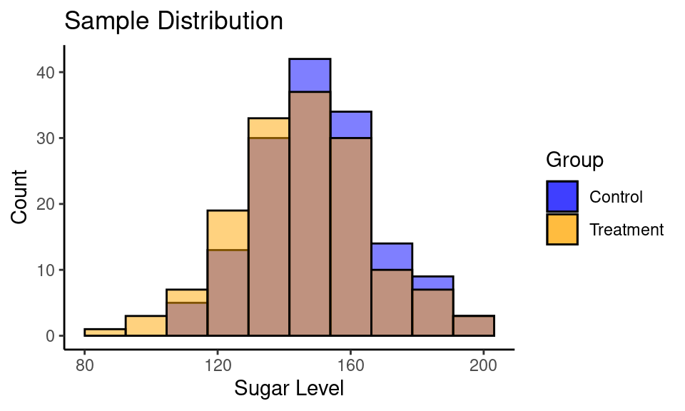
| Group | n | mean | std |
|---|---|---|---|
| Control | 150 | 150.44 | 18.08 |
| Treatment | 150 | 145.91 | 20.45 |
Calculate Cohen’s \(d\):
cohen.d(sample_control, sample_treatment)##
## Cohen's d
##
## d estimate: 0.2345 (small)
## 95 percent confidence interval:
## lower upper
## 0.00649 0.46253Case #2
set.seed(1)
sample_control <- rnorm(n = 150, mean = 150, sd = 20)
sample_treatment <- rnorm(n = 150, mean = 125, sd = 20)
ttest_results <- t.test(sample_treatment, sample_control,
                        alternative = "less")
ttest_results
##
## Welch Two Sample t-test
##
## data: sample_treatment and sample_control
## t = -11, df = 294, p-value <2e-16
## alternative hypothesis: true difference in means is less than 0
## 95 percent confidence interval:
## -Inf -20.85
## sample estimates:
## mean of x mean of y
## 125.9 150.4Code
ggplot() +
  geom_histogram(aes(sample_control, fill = "blue"), bins = 10,
                 color = "black", alpha = 0.5) +
  geom_histogram(aes(sample_treatment, fill = "orange", ), bins = 10,
                 color = "black", alpha = 0.5) +
  labs(title = "Sample Distribution",
       y = "Count",
       x = "Sugar Level") +
  scale_fill_manual(name = "Group", values = c("blue", "orange"),
                    labels = c("Control", "Treatment")) +
  theme_classic()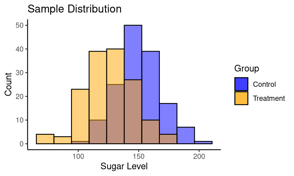
| Group | n | mean | std |
|---|---|---|---|
| Control | 150 | 150.44 | 18.08 |
| Treatment | 150 | 125.91 | 20.45 |
Calculate Cohen’s \(d\):
cohen.d(sample_control, sample_treatment)##
## Cohen's d
##
## d estimate: 1.271 (large)
## 95 percent confidence interval:
## lower upper
## 1.021 1.520Summary
I hope that all of these make sense now and you have a better picture of statistical hypothesis testing. The key point here is that low p-value is great, but not enough to make a decision (unless you specifically want to observe low effect size). And in order to avoid issues with low power and effect size you need to check what is the minimum sample size you need before the experiment.
In the first part I’ve described steps for the hypothesis testing framework, that could be updated now:
- Formulate the null and alternative hypotheses.
- Choose a proper test for a given problem.
- Set the significance level \(\alpha\) and \(\beta\).
- Find the minimum sample size needed to observe the desired effect size.
- Perform an experiment.
- Calculate the desired statistic using collected data and p-value associated with it.
- Calculate the effect size.
- Interpret the results in the context of a problem.
Kristoffer Magnusson has built some amazing visualizations that can help with building an intuition about Cohen \(d\) size and connection between power, sample size and effect size: Interpreting Cohen’s d Effect Size5, Understanding Statistical Power and Significance Testing6.
More examples of pwr package can be found at CRAN7.
References
Sullivan, G. M., & Feinn, R. (2012). Using Effect Size-or Why the P Value Is Not Enough. Journal of graduate medical education, 4(3), 279–282.
https://doi.org/10.4300/JGME-D-12-00156.1↩︎Sullivan, G. M., & Feinn, R. (2012). Using Effect Size-or Why the P Value Is Not Enough. Journal of graduate medical education, 4(3), 279–282.
https://doi.org/10.4300/JGME-D-12-00156.1↩︎Understanding Statistical Power and Significance Testing — an Interactive Visualization↩︎